Using Pheno-Ranker with TCGA Clinical Data

This guide explains how to use Pheno-Ranker with data from TCGA, obtained via the Genomic Data Commons Data Portal.

About this example

This example demonstrates how to process and use the data. It is not intended to yield relevant scientific conclusions.

Data Download

1. We are going to perform a data download by visiting the following link: Cohort Builder

2. In Project, select a few named TCGA. Then click in "CASES" and switch to Table View.

3. Next, click in TSV to download the data. You will likely end up with a file like: clinical.cohort.2025-06-02.tar.gz.

# Change the filename to match yours!
tar -xvf clinical.cohort.2025-06-02.tar.gz

The file we will use is clinical.tsv.

Why TSV and not JSON?

Pheno-Ranker works natively with JSON, so you could download JSON data. However, since the data often contains 2D-nested arrays, for this example it's easier to stick with TSV. The only caveat is that in the TSV, instead of all case-level data being consolidated into one object, we may have multiple rows per "case_id". Just be aware of that.

1. If you didn't select a specific cohort, you will end up with a TSV covering >45K cases and >100K rows. That might be a bit too much, so we will downsample to ~5K cases and replace empty values (and not reported) with "NA":

head -5001 clinical.tsv |sed -e "s/'--/NA/g" -e 's/no[tn] reported/NA/ig' > clinical_filtered.tsv

1. Now we will convert the TSV to a format ready for Pheno-Ranker, using the csv2pheno-ranker utility. Since the primary key case_id appears multiple times, we will generate a new primary key so the objects don't overwrite each other:

# Please change the path to match yours
../pheno-ranker/utils/csv2pheno_ranker/csv2pheno-ranker -i clinical_filtered.tsv --generate-primary-key --primary-key-name id -sep $'\t'

This will create two files:

clinical_filtered.json
clinical_filtered_config.yaml

Cohort Mode

We will begin with a simple calculation in cohort mode. In this run, we will also export intermediate files using --e tcga for later use.

Ensure that the pheno-ranker directory is set correctly:

time ../pheno-ranker/bin/pheno-ranker -r clinical_filtered.json -e tcga -config clinical_filtered_config.yaml --max-matrix-records-in-ram 10000

This calculation takes approximately 1:15 min (1 core on an Apple M2 Pro). The --max-matrix-records-in-ram 10000 flag improves efficiency by utilizing RAM, making the process about 2x faster.

Feel free to browse the miscellaneous data created as tcga*.

Since we have many variables that provide no value, we will add the following line to clinical_filtered_config.yaml. You can check which variables are used in tcga.glob_hash.json.

Simply open clinical_filtered_config.yaml with your favorite text editor and add:

# Set the regex to exclude variables matching a specific pattern
exclude_variables_regex: 'datetime|days_to_|cases.case_id|cases.submitter_id|demographic.demographic_id|demographic.submitter_id|diagnoses.diagnosis_id|diagnoses.submitter_id|project.project_id|treatments.protocol_identifier|treatments.submitter_id|treatments.treatment_id|age_of|treatment_dose|age_at|year_of_birth'

Quantitative data

In this exercise, we have decided to get rid of numerical data. In a real example, we would have created bins for quantitative variables.

Now run the calculation again:

time ../pheno-ranker/bin/pheno-ranker -r clinical_filtered.json -e tcga -config clinical_filtered_config.yaml --max-matrix-records-in-ram 10000  --exclude-terms id

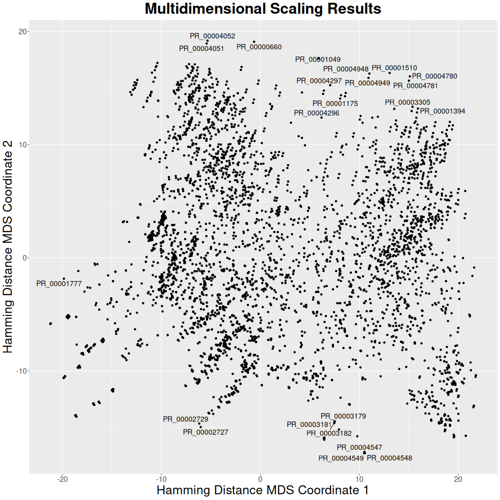
Since a 5,000 x 5,000 matrix is too large for a heatmap, we will use multidimensional scaling (mds.R script):

Rscript ../pheno-ranker/share/r/mds.R

This computation takes about 2:20 min (1 core on an Apple M2 Pro).

See R code

library(ggplot2)
library(ggrepel)

# Read in the input file as a matrix 
data <- as.matrix(read.table("matrix.txt", header = TRUE, row.names = 1, check.names = FALSE))

# Calculate distance matrix
#d <- dist(data)
#d <- 1 - data  # J-similarity to J-distance

# Perform multidimensional scaling
#fit <- cmdscale(d, eig=TRUE, k=2)
fit <- cmdscale(data, eig=TRUE, k=2)

# Extract (x, y) coordinates of multidimensional scaling
x <- fit$points[,1]
y <- fit$points[,2]

# Create data frame
df <- data.frame(x, y, label=row.names(data))

# Save image
png(filename = "mds.png", width = 1000, height = 1000,
    units = "px", pointsize = 12, bg = "white", res = NA)

# Create scatter plot
ggplot(df, aes(x, y, label = label)) +
  geom_point() +
  geom_text_repel(size = 5, # Adjust the size of the text
                  box.padding = 0.2, # Adjust the padding around the text
                  max.overlaps = 10) + # Change the maximum number of overlaps
  labs(title = "Multidimensional Scaling Results",
       x = "Hamming Distance MDS Coordinate 1",
       y = "Hamming Distance MDS Coordinate 2") + # Add title and axis labels
  theme(
        plot.title = element_text(size = 30, face = "bold", hjust = 0.5),
        axis.title = element_text(size = 25),
        axis.text = element_text(size = 15)) 

#dev.off()

Display plot

Patient Mode

Now we will attempt to match a given patient from the dataset to the rest. To do this:

../pheno-ranker/bin/pheno-ranker -r clinical_filtered.json -patients-of-interest PR_00000001

This will create the file PR_00000001.json.

Sorting by Jaccard index is recommended, since data completeness may be below 30%.

time ../pheno-ranker/bin/pheno-ranker -r clinical_filtered.json -t PR_00000001.json --config clinical_filtered_config.yaml -sort-by jaccard -max-out 5 --exclude-terms id

See Results

RANK	REFERENCE(ID)	TARGET(ID)	FORMAT	LENGTH	WEIGHTED	HAMMING-DISTANCE	DISTANCE-Z-SCORE	DISTANCE-P-VALUE	DISTANCE-Z-SCORE(RAND)	JACCARD-INDEX	JACCARD-Z-SCORE	JACCARD-P-VALUE	REFERENCE-VARS	TARGET-VARS	INTERSECT	INTERSECT-RATE(%)	COMPLETENESS(%)
1	PR_00000001	PR_00000001	CSV	8	False	0	-2.914	0.0017866	-2.8284	1.000	10.983	0.0000000	8	8	8	100.00	100.00
2	PR_00000906	PR_00000001	CSV	8	False	1	-2.810	0.0024794	-2.1213	0.875	9.549	0.0000000	7	8	7	87.50	100.00
3	PR_00003824	PR_00000001	CSV	9	False	2	-2.706	0.0034068	-1.6667	0.778	8.433	0.0000000	8	8	7	87.50	87.50
4	PR_00004720	PR_00000001	CSV	9	False	2	-2.706	0.0034068	-1.6667	0.778	8.433	0.0000000	8	8	7	87.50	87.50
5	PR_00002206	PR_00000001	CSV	9	False	2	-2.706	0.0034068	-1.6667	0.778	8.433	0.0000000	8	8	7	87.50	87.50

Let's take a look to the alignment related file. For this we will re-run but this time using the flag --align:

../pheno-ranker/bin/pheno-ranker -r clinical_filtered.json -t PR_00000001.json --config clinical_filtered_config.yaml -sort-by jaccard -max-out 5 --exclude-terms id --align

Feel free to browse align* files.

This is what looked like in my case for Rank 2 (yours may be different).

PR_00000001: 
  "cases.case_id" : "00016c8f-a0be-4319-9c42-4f3bcd90ac92"
PR_00000906: 
  "cases.case_id" : "01b7e692-d0cf-462f-9bbf-3ddb1572d025"

Inside alignment.txt (note that I omitted lines wth this pattern /^0 ----- 0 |/)

#RANK   REFERENCE(ID)   TARGET(ID)  FORMAT  LENGTH  WEIGHTED    HAMMING-DISTANCE    DISTANCE-Z-SCORE    DISTANCE-P-VALUE    DISTANCE-Z-SCORE(RAND)  JACCARD-INDEX   JACCARD-Z-SCORE JACCARD-P-VALUE REFERENCE-VARS  TARGET-VARS INTERSECT   INTERSECT-RATE(%)   COMPLETENESS(%) 
2   PR_00000906 PR_00000001 CSV      8  False      1     -2.810    0.0024794     -2.1213      0.875   9.549    0.0000000         7       8       7     87.50      100.00
--------------------------------------------------------------------------------
REF -- TAR
1 ----- 1 | (w:  1|d:  0|cd:  0|) cases.disease_type.Epithelial Neoplasms, NOS (Epithelial Neoplasms, NOS)
1 ----- 1 | (w:  1|d:  0|cd:  0|) cases.primary_site.Breast (Breast)
1 ----- 1 | (w:  1|d:  0|cd:  0|) demographic.gender.female (female)
1 ----- 1 | (w:  1|d:  0|cd:  0|) diagnoses.classification_of_tumor.metastasis (metastasis)
1 ----- 1 | (w:  1|d:  0|cd:  0|) diagnoses.morphology.8010/3 (8010/3)
1 ----- 1 | (w:  1|d:  0|cd:  0|) diagnoses.primary_diagnosis.Carcinoma, NOS (Carcinoma, NOS)
0 --xxx 1 | (w:  1|d:  1|cd:  1|) diagnoses.site_of_resection_or_biopsy.Thorax, NOS (Thorax, NOS)
1 ----- 1 | (w:  1|d:  0|cd:  1|) diagnoses.tissue_or_organ_of_origin.Breast, NOS (Breast, NOS)

Citation

If you use this information in your research, please cite the following:

1. The results shown here are in whole or in part based upon data generated by the TCGA Research Network: www.cancer.gov/tcga
2. Pheno-Ranker publication.