Using `Pheno-Ranker` with OMIM Data¶

This guide explains how to use Pheno-Ranker with data from the OMIM Database.

Data Download¶

Starting from version 1.02, Pheno-Ranker includes disease-based cohorts: one for the OMIM Database and another for the ORPHAnet Database.

Which data exchange formats

We provide two data exchange formats, PXF (Phenotype Exchange Format) and BFF (Beacon Friendly Format).

For more details on how these cohorts were created, refer to this repository. If you use this data in your research, please check the citation section.

If you installed the code via GitHub or Docker, the disease-based cohorts should already be available. Otherwise, follow these steps to download them. Ensure that wget and jq are installed:

sudo apt install wget jq

We assume that you have R installed and can install its required packages.

wget https://raw.githubusercontent.com/CNAG-Biomedical-Informatics/pheno-ranker/refs/heads/main/share/diseases/hpo/omim.pxf.json.gz

Here, we will use the PXF version of the disease-based cohort.

Analytics¶

zcat omim.pxf.json.gz | jq 'length'

The cohort consists of 6,471 diseases. Each disease is represented as a PXF containing a list of phenotypicTerms.

From this point onward, we assume that the pheno-ranker directory is located at ../. Please adjust the path accordingly.

To analyze the distribution of terms across patients, we will use a Perl script.

See Perl code

#!/usr/bin/perl
use strict;
use warnings;
use JSON::XS;

# Read from STDIN only
if (-t STDIN) {  # Check if STDIN is empty (no piped input)
    print STDERR "Usage: zcat input.json.gz | $0\n";
    print STDERR "       cat input.json | $0\n";
    exit 1;
}

# Read the entire JSON content from STDIN
my $json_text = do {
    local $/;
    <STDIN>;
};

# Decode JSON
my $json = JSON::XS->new->utf8->decode($json_text);

# Ensure the decoded JSON is an array reference
die "Input JSON is not an array.\n" unless ref($json) eq 'ARRAY';

# Print CSV header
print "key,count\n";

# Iterate through each object in the array
foreach my $obj (@$json) {
    # Ensure the current element is an object with an 'id' field
    next unless ref($obj) eq 'HASH' && exists $obj->{id};

    my $id = $obj->{id};
    my $count = 0;

    # Check if 'phenotypicFeatures' exists and is an array
    if (exists $obj->{phenotypicFeatures} && ref($obj->{phenotypicFeatures}) eq 'ARRAY') {
        $count = scalar @{ $obj->{phenotypicFeatures} };
    }

    # Print the CSV line
    print "\"$id\",$count\n";
}

zcat omim.pxf.json.gz | ./count_phenotypicFeatures.pl > counts.csv

Now, we will use R to plot a histogram.

See R code

# Load required packages
library(ggplot2)

# Read the CSV file into a data frame
df <- read.csv("counts.csv")

# Calculate the average and median counts
average_count <- mean(df$count)
median_count <- median(df$count)

# Generate the histogram and add vertical lines for the average and median
plot <- ggplot(df, aes(x = count)) +
  geom_histogram(binwidth = 1, fill = "steelblue", color = "black") +
  geom_vline(aes(xintercept = average_count), color = "black", linetype = "dashed", linewidth = 1) +
  geom_vline(aes(xintercept = median_count), color = "red", linetype = "dashed", linewidth = 1) +
  labs(title = "Distribution of Element Counts per Object",
       x = "Number of Elements",
       y = "Frequency") +
  theme_minimal() +
  annotate("text", x = average_count + 0.5, y = Inf, label = paste("Mean:", round(average_count, 2)), vjust = 2) +
  annotate("text", x = median_count - 0.5, y = Inf, label = paste("Median:", round(median_count, 2)), vjust = 2, color = "red")

# Save the plot as a PNG file
ggsave("histogram_with_mean_median.png", plot = plot, width = 8, height = 6, dpi = 300)

# Print confirmation
cat("Histogram saved as histogram_with_mean_median.png\n")

Display plot

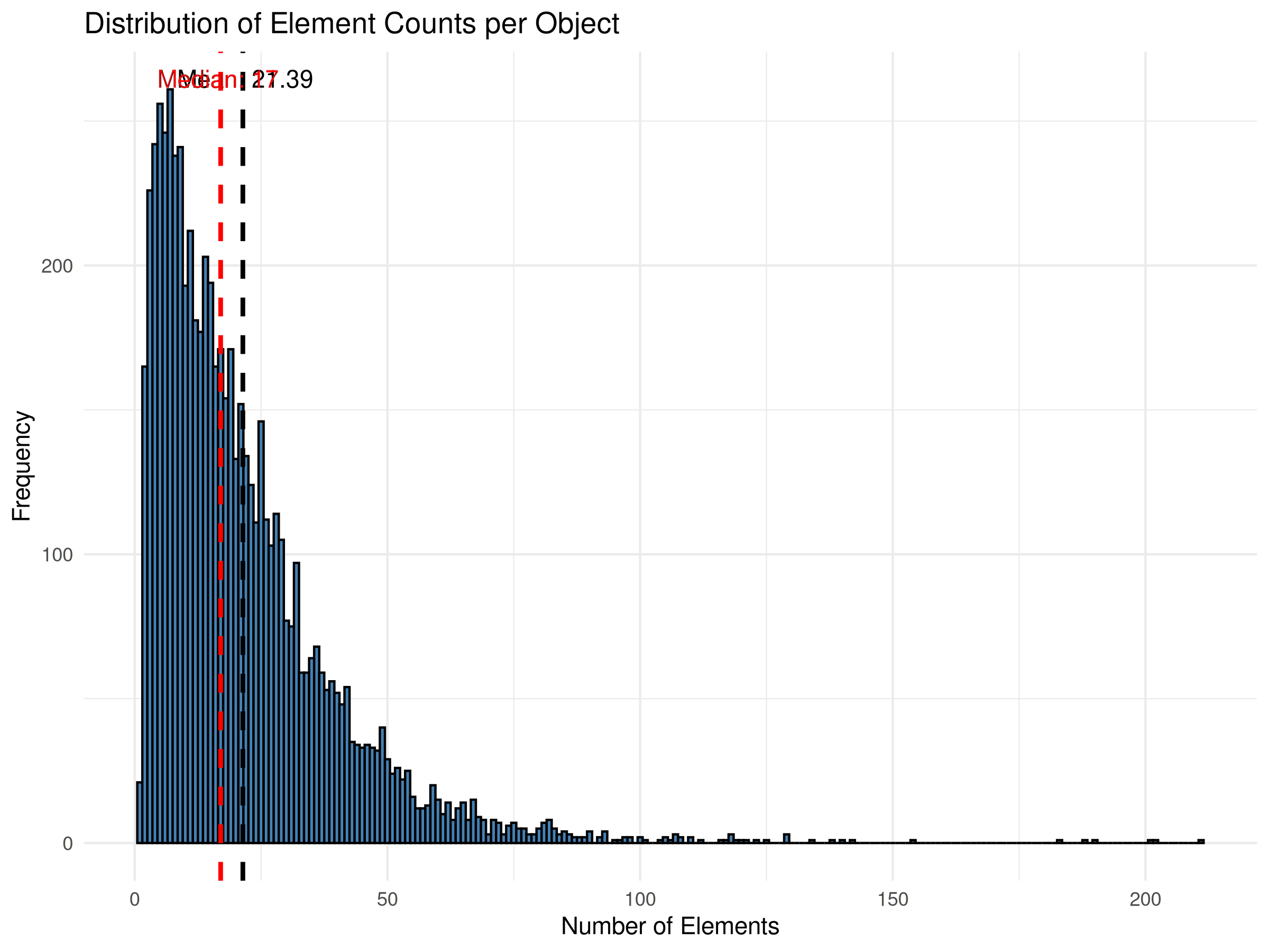
Based on the median, the Completeness of the Phenopackets Corpus is approximately 71% (12/17).

Cohort Mode¶

We begin with a simple calculation in cohort mode. In the run, we will also export intermediate files using --e omim for later use. From now on, we will focus on phenotypicFeatures terms, which we aim to use for patient classification.

Ensure that the pheno-ranker directory is set correctly.

time ../pheno-ranker/bin/pheno-ranker -r omim.pxf.json.gz --include-terms phenotypicFeatures --max-matrix-items-in-ram 10000 -e omim

This calculation takes approximately 1 min 40 sec (1 core @ Apple M2 Pro). The --max-matrix-items-in-ram 10000 flag increases efficiency by using RAM, making the process 2x faster.

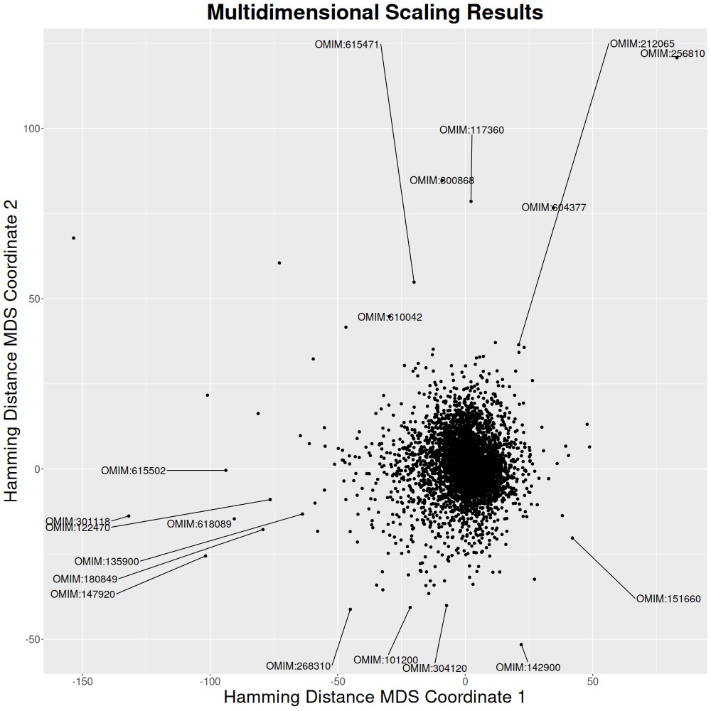
Since a 6,471 × 6,471 matrix is too large for a heatmap, we will use multidimensional scaling (mds.R script).

Rscript ../pheno-ranker/share/r/mds.R

This computation takes about 5 minutes (1 core @ Apple M2 Pro).

See R code

library(ggplot2)
library(ggrepel)

# Read in the input file as a matrix 
data <- as.matrix(read.table("matrix.txt", header = TRUE, row.names = 1, check.names = FALSE))

# Calculate distance matrix
#d <- dist(data)
#d <- 1 - data  # J-similarity to J-distance

# Perform multidimensional scaling
#fit <- cmdscale(d, eig=TRUE, k=2)
fit <- cmdscale(data, eig=TRUE, k=2)

# Extract (x, y) coordinates of multidimensional scaling
x <- fit$points[,1]
y <- fit$points[,2]

# Create data frame
df <- data.frame(x, y, label=row.names(data))

# Save image
png(filename = "mds.png", width = 1000, height = 1000,
    units = "px", pointsize = 12, bg = "white", res = NA)

# Create scatter plot
ggplot(df, aes(x, y, label = label)) +
  geom_point() +
  geom_text_repel(size = 5, # Adjust the size of the text
                  box.padding = 0.2, # Adjust the padding around the text
                  max.overlaps = 10) + # Change the maximum number of overlaps
  labs(title = "Multidimensional Scaling Results",
       x = "Hamming Distance MDS Coordinate 1",
       y = "Hamming Distance MDS Coordinate 2") + # Add title and axis labels
  theme(
        plot.title = element_text(size = 30, face = "bold", hjust = 0.5),
        axis.title = element_text(size = 25),
        axis.text = element_text(size = 15)) 

#dev.off()

Display plot

Graph Representation¶

To generate a graph visualization, we use a subset of 50 diseases for faster execution.

zcat omim.pxf.json.gz | jq -c '.[]' | shuf -n 50 | jq -s '.' > omim_small.json
../pheno-ranker/bin/pheno-ranker -r omim_small.json -include-terms phenotypicFeatures --cytoscape-json omim_cytoscape.json

Display plot

Patient Mode¶

We will attempt to match patient PMID_35344616_A2 from the Phenopackets Corpus to its disease (OMIM:268310) in OMIM. See the Phenopackets Corpus tutorial for instructions on obtaining a PXF file for the patient.

Sorting by Jaccard index is recommended, as data completeness is below 30%. From the top three, selecting by INTERSECT-RATE(%) ranks the match at 1.

../pheno-ranker/bin/pheno-ranker -r omim.pxf.json.gz -t PMID_35344616_A2.json -include-terms phenotypicFeatures -sort-by jaccard -max-out 5

See Results

RANK	REFERENCE(ID)	TARGET(ID)	FORMAT	LENGTH	WEIGHTED	HAMMING-DISTANCE	DISTANCE-Z-SCORE	DISTANCE-P-VALUE	DISTANCE-Z-SCORE(RAND)	JACCARD-INDEX	JACCARD-Z-SCORE	REFERENCE-VARS	TARGET-VARS	INTERSECT	INTERSECT-RATE(%)	COMPLETENESS(%)
1	OMIM:180700	PMID_35344616_A2	PXF	77	False	52	0.111	0.5440913	3.0769	0.325	10.784	71	31	25	80.65	35.21
2	OMIM:616894	PMID_35344616_A2	PXF	64	False	44	-0.397	0.3457285	3.0000	0.312	10.359	53	31	20	64.52	37.74
3	OMIM:268310	PMID_35344616_A2	PXF	107	False	76	1.634	0.9488308	4.3503	0.290	9.563	107	31	31	100.00	28.97
4	OMIM:618529	PMID_35344616_A2	PXF	53	False	39	-0.714	0.2375690	3.4340	0.264	8.670	36	31	14	45.16	38.89
5	OMIM:616331	PMID_35344616_A2	PXF	84	False	64	0.872	0.8084460	4.8008	0.238	7.759	73	31	20	64.52	27.40

This process takes ~10 seconds. For a much faster approach using precomputed data, run:

../pheno-ranker/bin/pheno-ranker -prp omim -t PMID_35344616_A2.json -include-terms phenotypicFeatures -sort-by jaccard -max-out 5

With precomputed data, the calculation takes only 0.5 seconds while yielding identical results.

Citation¶

If you use this information in your research, please cite the following:

Using Pheno-Ranker with OMIM Data¶

Data Download¶

Analytics¶

Cohort Mode¶

Graph Representation¶

Patient Mode¶

Citation¶

Using `Pheno-Ranker` with OMIM Data¶